Abstract
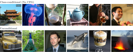
Iterative sampling in diffusion models during inference can lead to error accumulation due to exposure bias. The denoiser is trained on real training images interpolated with noise, but at inference its inputs are constructed from its own imperfect predictions from the earlier steps, something it has never seen at training time. This might be one reason diffusion models often struggle without additional help, such as CFG. In this paper, we introduce a correction step for diffusion models which attempts to reduce this training-inference gap. The corrector takes the base model’s own prediction as input and is trained against the same ground-truth target as the base model. This makes correction an explicit learning task, with training inputs provided by the base model. During sampling, at each denoising step, we iteratively refine the denoiser’s clean-sample prediction. This allows us to correct predictions at intermediate denoising steps, preventing early artifacts from persisting into the final sample. We find that applying correction beyond the single step supervised during training is key to the significant quality gains. This simple framework leads to substantial improvement in sample quality while largely preserving diversity. We extensively evaluate our method across widely used architectures, including DiT, SiT, and JiT. Our method substantially improves upon previously reported FID scores for unguided generation and unconditional generation. Our method achieves performance competitive with classifier-free guidance (CFG), and combining correction with CFG further improves diversity and reduces oversaturation typical of CFG. Finally, we show that the additional inference cost of correction can be amortized by distilling the refined predictions back into the base diffusion model, retaining the quality gains without additional inference-time overhead.
Uncurated samples
Loading samples…
Diffusion models often generate poor-quality images without guidance
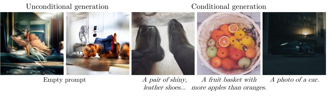
Without guidance, diffusion models produce poor-quality samples even in recent large-scale models such as FLUX.2 Klein 9B. This has been a long-standing issue in diffusion-based image generation. Diffusion models generate good images only with classifier-free guidance.1
Early structural errors compound over later denoising steps
During training, the denoiser learns from noisy real images. During sampling, it receives intermediate states produced by its own imperfect predictions. This training–inference gap can let errors accumulate. In the example below, an unnatural mouth structure appears early; later denoising mainly adds detail without repairing it.
1Train the denoiser
Training inputs are real images mixed with noise. Given a noisy image, the denoiser predicts the clean image, and an L2 loss compares the prediction with the target.
2Sample from noise
During sampling there is no real image. We start from noise, and each denoising step mixes the prediction into the next, less noisy input.
3The training–inference gap
With a perfect denoiser, sampling inputs would follow exactly the same distribution as training inputs. A learned denoiser makes small errors, and each error is fed into the next input, so sampling inputs can drift away from those seen during training.
4Early errors are carried forward
Here, a broken mouth appears early. Each prediction feeds the next input, so the inputs drift as in the schematic above, and later steps add teeth, eyes and texture while keeping the broken structure.
Sampling: the Fig. 3(a) sample from the paper (SiT-REPA-XL/2, ImageNet 256×256, no guidance, 250 steps; selected steps shown). Training: an ImageNet training image of the same class, noised at t = 0.6. Noisy inputs are shown as decoded latents. Step 3 is a schematic.
Method
How do we do this? The method is very simple.
1Train the denoiser
Given a noisy image, the denoiser predicts the clean image. An L2 loss compares the prediction with the target.
2Train the corrector
The corrector refines the denoiser’s prediction toward the same clean target. Stop-gradient (sg) keeps the correction loss from training the denoiser.
3Sample from noise
We follow one sample through its 250 denoising steps. Steps 1–32 are not shown.
4Denoise, then correct K times
The denoiser makes a prediction. At the same noise level, the corrector then refines that prediction K = 8 times.
5Take the denoising step and repeat
The corrected prediction gives the next, less noisy input, and the same loop runs again (shown here at step 40).
6Later steps
The same loop runs at every step. Later, at step 79, the prediction is already sharp and the corrections refine it further.
7Final sample
The remaining steps run the same way and end in the final sample.
Overall framework: We introduce a corrector trained to refine the base denoiser's prediction toward the same clean target used in the denoising loss (top row). During sampling, we iteratively correct the denoiser's prediction at each denoising step (bottom row).
Improve sample quality with iterative correction
Although the framework is simple, it's highly effective. Applying more corrections at each denoising step during inference produces significantly higher-quality images, with cleaner structures and fewer artifacts.
The corrected sampling trajectory starts from the same initial noise. Correction can change the coarse structure of a prediction before the sampler moves to the next noise level. Here, repeated refinement produces a coherent mouth and face.
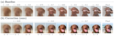
Top: baseline trajectory, K=0. Bottom: one corrected trajectory, K=8. Each triplet shows the prediction before correction (k=0), after one correction (k=1), and after eight corrections (k=8) at a fixed noise level.
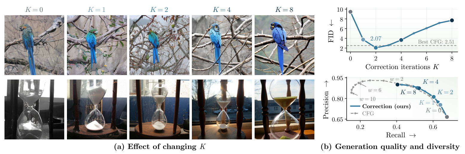
Left: SiT-REPA final samples at different K. Right: DiT FID and precision–recall, evaluated on 50K images per setting.
Correction significantly improves sample quality
In this work, we propose a method that enables diffusion models to generate high-quality, realistic samples without relying on guidance. We tested our method on four widely used baselines: DiT, SiT, SiT-REPA, and JiT. Our method significantly improves FID over the unguided baseline across all four models, using the same or a smaller inference budget than CFG.
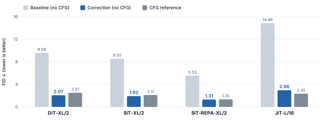
Class-conditional ImageNet-256, FID on 50K samples, approximately 250 network evaluations per image (including denoiser and corrector calls for correction, and unconditional calls for CFG). We keep the number of network evaluations for correction no larger than that for CFG. See the paper for each model's settings.
Correction has better diversity and less oversaturation
If it's comparable to CFG, why don't we just use CFG? CFG has two well-known weaknesses: mode collapse and oversaturation.
- Mode collapse: CFG often substantially reduces the diversity of generated samples. This usually appears as boring or repetitive layouts, poses, and styles for a given text prompt.
- Oversaturation: CFG often makes sample colors highly saturated, contributing to the "AI look" of many text-to-image diffusion models.
Our correction avoids both issues in these examples. Below, we compare increasing the CFG scale with increasing the number of corrections:
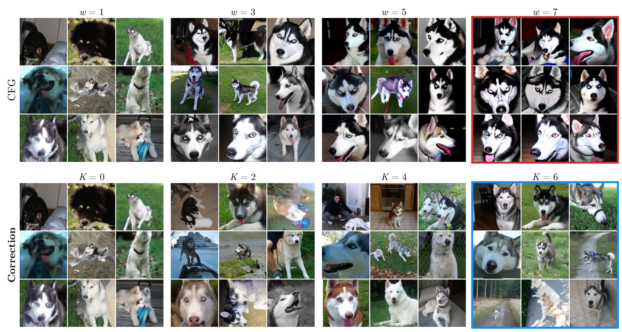
SiT-REPA-XL/2, same class and initial noise, approximately matched NFE. Top: increasing CFG scale w. Bottom: increasing correction K without CFG.
Increasing CFG can push samples toward similar close-up portraits and oversaturated colors. Correction preserves more varied poses, framings, and backgrounds while producing sharp, coherent images.
Text-to-image results
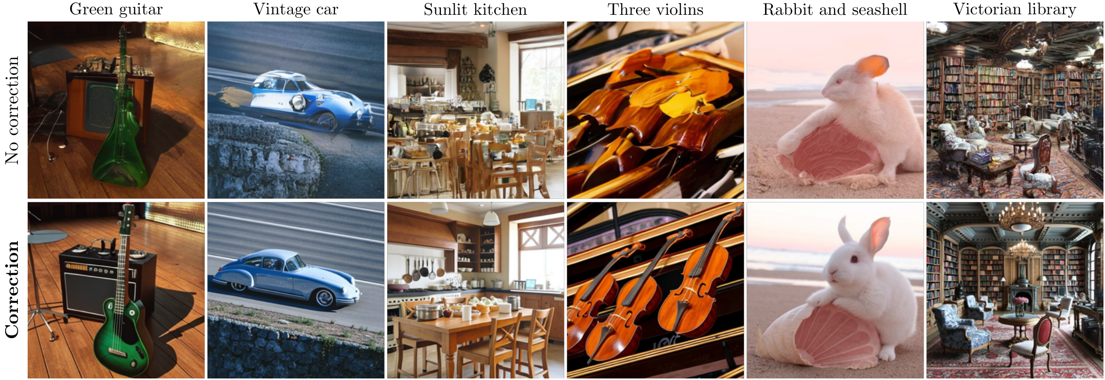
Does our method work beyond ImageNet generation? Yes. We test it on NanoGen, a unified diffusion transformer implementation for ImageNet and text-to-image generation. The base model is pretrained on BLIP-3o's Short-Caption, Long-Caption, and JourneyDB subsets, whose original releases contain approximately 36M image–text pairs in total. Below, we show samples without guidance (top row) and with correction (bottom row). Correction significantly improves the samples, producing cleaner object structures.
Correction combined with CFG improves diversity and realism
We can combine CFG with correction to benefit from both. Adding correction can reduce the AI look, oversaturated or overcooked colors, and loss of diversity caused by CFG.
These text-to-image samples with CFG have a pronounced AI look and limited diversity: all the benches face forward.
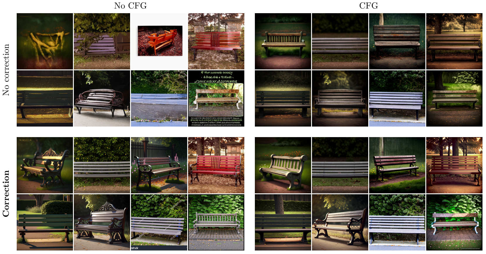
Prompt: “a photo of a bench.” All four groups use the same eight seeds and 50 denoising steps. Columns: no CFG (w=1), CFG (w=6). Rows: no correction (K=0), correction (K=6).
Applying correction to the CFG prediction during denoising makes the samples more diverse, with more varied viewpoints, and more realistic.
Correction alone also generates high-quality samples with greater diversity and much less oversaturation; many now look like natural images. We can control diversity and prompt adherence by adjusting the CFG scale while continuing to apply correction during sampling. The corrected samples look better than the baseline samples both with and without CFG.
We also conduct a human study to assess whether people perceive improvements in sample quality and diversity with correction. This is practically important for researchers and developers building large-scale text-to-image diffusion models. Across 80 GenEval single-object prompts, we collected 800 responses per criterion (1,600 in total), with 10 judgments per prompt for each criterion, through Rapidata. The baseline uses CFG only, at DiffusionBench's default CFG scale.
| Criterion | CFG + correction | CFG only |
|---|---|---|
| Quality | 60.75% | 39.25% |
| Diversity | 60.25% | 39.75% |
Why does correction help?
Correction is simple, and it works across models. But why does it work so well? We look at two questions here; more analyses are in Section 4 (Discussion) of the paper.
The gain comes from applying correction iteratively
A natural suspicion is that correction simply adds parameters. To test this, we train two models from scratch with the same total number of transformer layers (LightningDiT, ImageNet 256×256, 80K updates): a 28-layer denoiser, and a 14-layer denoiser paired with a 14-layer corrector. With one correction per denoising step, the pair performs about the same as the deeper denoiser (FID 8.74 vs. 8.93).
The gain comes from repeating the correction. Applying the same corrector three times per step, with half as many denoising steps so that the compute budget is unchanged, lowers FID to 5.66. Correction is not merely a way to add parameters or inference compute.
1A deeper denoiser
The baseline is one 28-layer denoiser, run for 240 denoising steps: 6,720 layer evaluations in total. FID 8.93.
2Split it in two, correct once
A 14-layer denoiser plus a 14-layer corrector has the same 28 layers per step. With one correction per step, it performs about the same: FID 8.74.
3Correct three times, take half the steps
Applying the corrector three times makes each step twice as deep, so we take half as many steps (120). The total compute is unchanged: 6,720 layer evaluations.
4Same compute, much better FID
With the same corrector applied three times, FID drops to 5.66. The gain comes from repeating the correction, not from more parameters or compute.
LightningDiT on ImageNet 256×256, trained from scratch for 80K updates (675M vs. 681M parameters); FID on 8K samples, no guidance. Block width shows the number of transformer layers.
It narrows the training–inference gap
Surprisingly, correction does not lower the denoising error, the squared error used for training. After three or more corrections, the error is higher than the base denoiser’s. The catch is where this error is measured: on noisy training inputs, made from real images. During sampling, the denoiser instead sees states built from its own earlier predictions, as shown above, and what matters for generation is how well it handles those states. We hypothesize that correction helps by keeping them closer to what the denoiser saw during training.
To test this, we train a classifier to tell the two apart: is this noisy state from training, or from a sampling run? If it cannot do better than a coin flip, the two distributions are indistinguishable. For a standard SiT model, the classifier separates them easily, especially at low noise levels where errors have accumulated. One correction makes the task harder, and four corrections harder still. Correction narrows the training–inference gap, even though the error on training inputs goes up.
1Two kinds of noisy states
Training states are real images plus noise. Sampling states are built from the model’s own earlier predictions. To us, they look alike.
2Can a classifier tell them apart?
We train a classifier to guess where a noisy state came from. If it can only guess (AUROC 0.5), there is no gap. The easier it tells them apart, the larger the gap.
3Without correction: easy to tell apart
For a standard SiT model, the classifier separates the two easily, especially near the data, where errors have accumulated over the sampling run.
4One correction
With one correction per step, the sampling states become harder to tell apart from training states.
5Four corrections: a smaller gap
With four corrections, they are harder still to tell apart. Correction narrows the training–inference gap.
Held-out AUROC of a classifier trained on 100K intermediate states of SiT, per noise level (data from the paper’s Fig. on classifier two-sample tests; binary cross-entropy shows the same trend in the paper). Near pure noise all settings are close to chance. Example noisy states in steps 1–2 are decoded latents for illustration only.
Citation
Acknowledgments
We would like to thank Konpat Preechakul for valuable insights and feedback, as well as Michael Gharbi for insightful discussions, and Nicolas Dufour for providing detailed feedback on the manuscript. We are grateful to A. Sophia Koepke, Anne Harrington, Amil Dravid, Jorge Diaz Chao, Isabella Yu, Yutong Bai, Yong-Hyun Park, Sangyoon Lee, Sihyun Yu, Susung Hong, Joonghyuk Shin, Gyuseong Lee, and Sanghyun Lee for helpful discussions. This work was supported, in part, by NSF IIS-2403305 and ONR MURI grants.
Other approaches include alternative guidance methods, reinforcement learning, and supervised fine-tuning on a small, high-quality dataset. None has fully satisfied us: RL-based approaches typically require external models, while supervised fine-tuning can sacrifice substantial diversity.↩